Computers can be used to produce art, but can they produce art on their own?
Yes. Yes they can, and they have been doing exactly that for quite some time. Your smartphone can use a neural network to imitate the style of long-dead master painters and apply it to pictures of your cats.
But you don't need to go that far to produce interesting results.
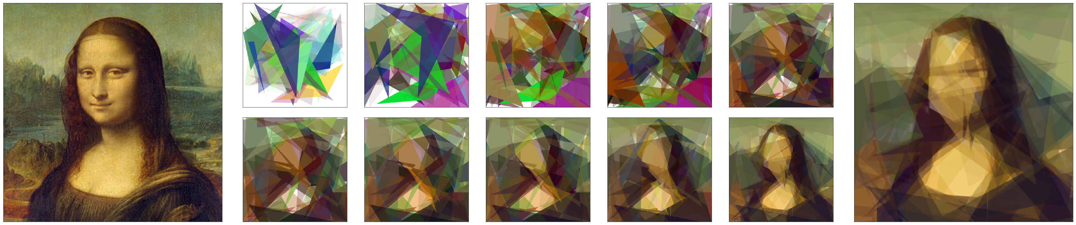
EvoLisa is a comparatively simple example of generative art. It uses a bunch of overlapping, semi-transparent polygons to approximate a picture - producing images that are, if not artistic, at least interesting to look at.
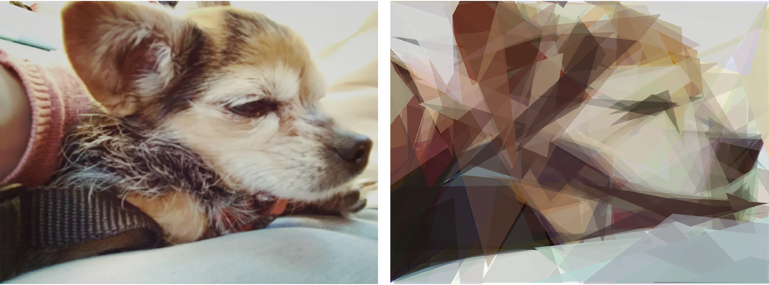
But what does the computer know about art? How does it decide which colors are best, which shapes to use? That's easy. It has zero knowledge and inifinite patience.
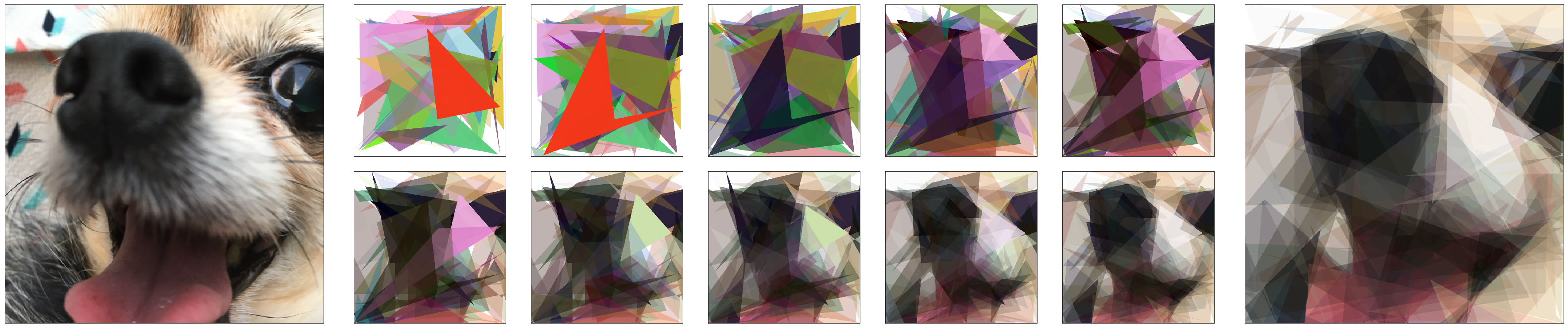
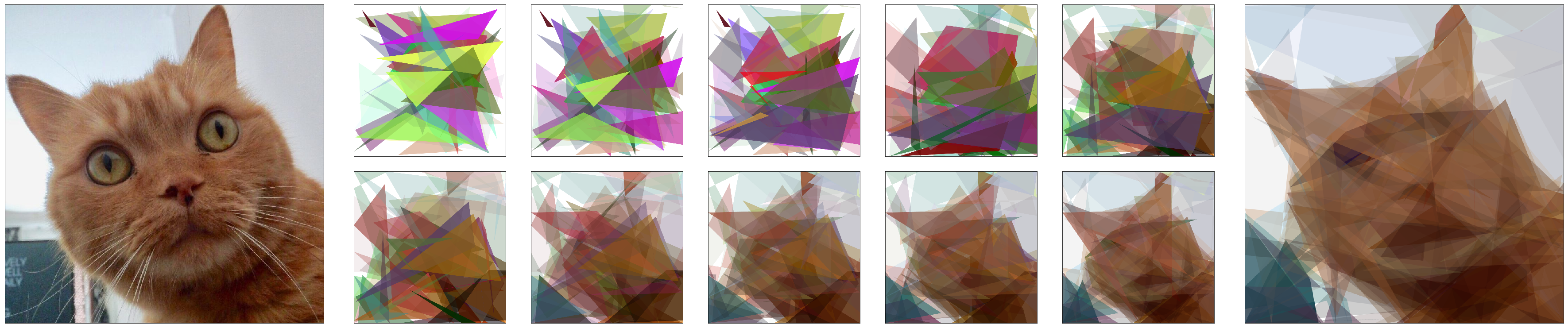
So it tries. And fails. So it changes its approach slightly, and tries again. And again. And again and again and again, slowly iterating its approach. Give it enough time, and you start to get recognizable results.
Implementing a search algorithm
EvoLisa is an example of search algorithm - an algorithm that looks for optimal results in the space of all possible solutions to a given problem. That is, given all possible combinations of polygons, the algorithm searchs for the one that is the most similar to the original image.
Now there are many ways of making this search. In this case we are iterating over incremental random changes to a single solution, so we are talking about a Stochastic Hill Climbing algorithm.
A search algorithm has three critical points: a data structure that holds the data we are optimizing. a means of generating new solutions. * a method that gives a score to our solutions.
We can see how they fit together if we sketch the algorithm in pseudocode:
original = get image from file
polygons = generate a bunch of random polygons

loop:
    new_polygons = make a small change to polygons
    if new_polygons is closer to original than polygons:
        replace polygons with new_polygons
The algorithm's performance will depend on the design choices and tradeoffs we make regarding these three points.
What's an image? A miserable pile of arrays
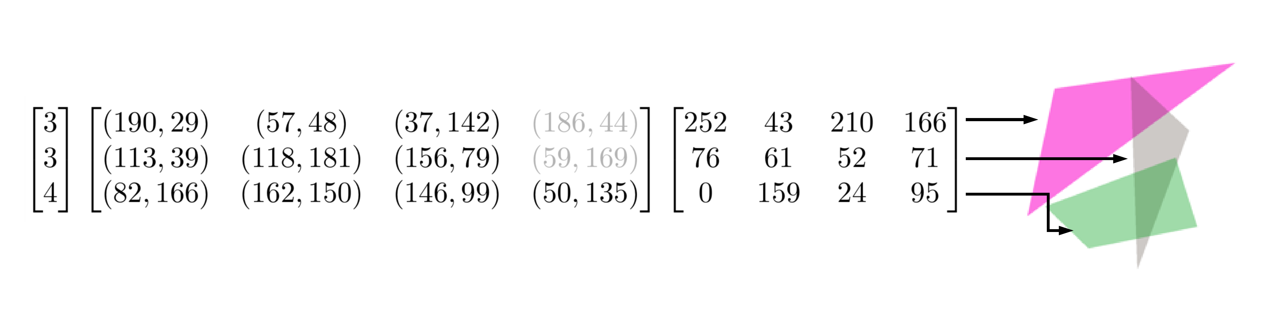
Each one of the polygons that define our image is defined by two things: a list of (x, y) points that define the outline. a RGBA value for the fill color and transparency.
We want to have a variable number of points per polygon, but it should be easier (and probably faster) to work with arrays of fixed length. We'll add a third value containing the number of points of our polygon - this way we can have outlines of fixed length but only used the points we need.
In the image we can see three randomly generated shapes and the corresponding arrays for the number of points, coordinates and colors.
All these values will be stored inside numpy arrays because they are pretty standard, reasonably fast, and well suited to our purpouses. For example, there are a number of functions for generating random arrays that will be useful when initializing our shapes.
Trying something new
Our algorithm finds better solutions by making small changes to the current one and seeing if there is any improvement. The kind of changes we make will determine what kind of results are possible, so it's important to define them carefully.
This implementation randomly applies one of the following changes to a random polygon in the set: Displace one of the points of the polygon by a random amount in the XY axis. Displace the whole polygon by a random amount in the XY axis. Change the drawing order of the points - each point is connected to the next one, so by changing the order we change the shape. Add or remove a point from the polygon. Change the color by a random amount in the RGB axis. Change the transparency by a random amount.
It's important to make sure that the changes don't produce invalid solutions. All points must be within the boundaries of the image, all color values must stay within the 0-255 range, and the number of points can't be more or less than a user-defined amount.
Does this look like a face to you?
The last thing we need is a function that tells us how close we are to the original image. In this case we compare the image resulting from our polygon set with the original, in a pixel-by-pixel basis. We can add the absolute values of this difference for each pixel to get a value that represents how different the two images are. This value can be normalized over the number of pixels to produce a human-readable value, but it's not relevant to the algorithm because the size of the images remains constant between iterations.
def error_abs(a, b):
    return np.abs(np.subtract(a, b, dtype=np.dtype('i4'))).sum()
I stumbled upon a pitfall here. Image arrays are composed by unsigned 8-bit numbers because they only contain positive values between 0 and 255. If we try to substract then normally, we get an array of the same type - with the negative values overflowing to positive again. This can lead to unexpected results - in my case, I found out when the algorithm started generating deep blue cats.
Smaller is faster
With all this three pieces, the algorithm is ready to run. But the goal wasn't getting it to run, it was getting it to run fast.
So let's take our algorithm to a stroll with Line Profiler to see where it's wasting it's time.
    Time  % Time    Line Contents
===============================================================================
                    def iterate(shapes, points, colors, score):
   170.0     0.2        n_shapes, n_points, n_colors = changes(
                            shapes, points, colors)
 41315.0    46.4        n_image = np.array(draw_image(
                            width, height, n_shapes, n_points, n_colors))
 47594.0    53.4        new_score = error_abs(internal, new_image)

     4.0     0.0        if new_score < score:
                            return n_shapes, n_points, n_colors, n_score
     1.0     0.0        return shapes, points, colors, score
We can see that two lines take up 99.8% of processing time: The generation of a new image from the set of shapes takes up 46.4% of the time. Calculating the difference between images takes up 53.4% of the time.
Both lines heavily depend on the input image size. That is, if the image is bigger the algorithm will take longer. What can we do about it?
We can make a tradeoff - speed por precission. That is, we can take the original image, scale it down to a more manageable size, and work with that.
If we scale down the image by a factor of eight:
    Time  % Time    Line Contents
===============================================================================
                    def iterate(shapes, points, colors, score):
  1293.0    18.2        n_shapes, n_points, n_colors = changes(
                            shapes, points, colors)
  3444.0    48.5        n_image = np.array(draw_image(
                            width, height, n_shapes, n_points, n_colors))
  2319.0    32.6        new_score = error_abs(internal, new_image)

    47.0     0.7        if new_score < score:
                            return n_shapes, n_points, n_colors, n_score
     2.0     0.0        return shapes, points, colors, score
We can see that the times are an order of magnitude lower or better than before. Of course the images we get won't be as good as before, but we'll get them in a manageable amount of time.
The scaling factor is also configurable, so the tradeoff can be configured depending on the desired results. It'd be possible to improve both precission and speed by modifying the scaling factor on the fly - improving precision as the algorithm converges.
Enough numbers, let's see some results

Try this at home kids!
The source code for this project is available in github.